Getting Started
Demos
Notebooks: The notebooks provide a simple and friendly way to get into Caiman and understand its main characteristics. They are located in the
demos/notebooks. To launch one of the jupyter notebooks, activate your conda caiman environment, enter the caiman_data directory, and then:jupyter lab --ZMQChannelsWebsocketConnection.iopub_data_rate_limit=1.0e10
and select the notebook from within Jupyter’s browser. The argument provided will prevent any output from being lost while using a notebook
demo files are also found in the demos/general subfolder. We suggest trying demo_pipeline.py first as it contains most of the tasks required by calcium imaging. For behavior use demo_behavior.py
Basic Structure
We recently refactored the code to simplify the parameter setting and usage of the various algorithms. The code now is based revolves around the following objects:
params: A single object containing a set of dictionaries with the parameters used in all the algorithms. It can be set and changed easily and is passed into all the algorithms.MotionCorrect: An object for motion correction which can be used for both rigid and piece-wise rigid motion correction.cnmf: An object for running the Caiman batch algorithm either in patches or not, suitable for both two-photon (CNMF) and one-photon (CNMF-E) data.online_cnmf: An object for running the Caiman online (OnACID) algorithm on two-photon data with or without motion correction.estimates: A single object that stores the results of the algorithms (batch, online) in a unified way that also contains plotting methods.
To see examples of how these methods are used, please consult the demos.
Parameters
Caiman gives you access to a lot of parameters and lets you adapt the analysis to your data. Parameters are stored in
the params object in a set of dictionaries, sorted by the part of the analysis they are used in:
data: General params describing the dataset like dimensions, decay time, filename and framerateinit: Parameters for component initialization like neuron sizegSig, patch size etc.motion: motion correction parameters (max shift size, patch size etc.)online: Parameters specific for the online OnACID algorithmquality: Parameters for component evaluation (spatial correlation, SNR and CNN)spatial: Parameters used in detection of spatial componentstemporal: Parameters used in extraction of temporal components and deconvolution
Of these parameters, most have a default value that usually does not have to be adjusted. However, some parameters are crucial to be adapted to the specific dataset for proper analysis performance:
fnames: List of paths to the file(s) to be analysed. Memmap and hdf5 result files will be saved in the same directory.fr: Imaging frame rate in frames per second.decay_time: Length of a typical transient in seconds.decay_timeis an approximation of the time scale over which to expect a significant shift in the calcium signal during a transient. It defaults to0.4, which is appropriate for fast indicators (GCaMP6f), slow indicators might use 1 or even more. However, decay_time does not have to precisely fit the data, approximations are enough.p: Order of the autoregressive model.p = 0turns deconvolution off. If transients in your data rise instantaneously, setp = 1(occurs at low sample rate or slow indicator). If transients have visible rise time, setp = 2. If the wrong order is chosen, spikes are extracted unreliably.nb: Number of global background components. This is a measure of the complexity of your background noise. Defaults tonb = 2, assuming a relatively homogeneous background.nb = 3might fit for more complex noise,nb = 1is usually too low. Ifnbis set too low, extracted traces appear too noisy, ifnbis set too high, neuronal signal starts getting absorbed into the background reduction, resulting in reduced transients.merge_thr: Merging threshold of components after initialization. If two components are correlated more than this value (e.g. when during initialization a neuron was split in two components), they are merged and treated as one.rf: Half-size of the patches in pixels. Should be at least 3 to 4 times larger than the expected neuron size to capture the complete neuron and its local background. Larger patches lead to less parallelization.stride: Overlap between patches in pixels. This should be roughly the neuron diameter. Larger overlap increases computational load, but yields better results during reconstruction/denoising of the data.K: Number of (expected) components per patch. Adapt torfand estimated component density.gSig: Expected half-size of neurons in pixels [rows X columns]. CRUCIAL parameter for proper component detection.method_init: Initialization method, depends mainly on the recording method. Usegreedy_roifor 2p data,corr_pnrfor 1p data, andsparse_nmffor dendritic/axonal data.ssub/tsub: Spatial and temporal subsampling during initialization. Defaults to 1 (no compression). Can be set to 2 or even higher to save resources, but might impair detection/extraction quality.
Component evaluation
The quality of detected components is evaluated with three parameters:
Spatial footprint consistency (
rval): The spatial footprint of the component is compared with the frames where this component is active. Other component’s signals are subtracted from these frames, and the resulting raw data is correlated against the spatial component. This ensures that the raw data at the spatial footprint aligns with the extracted trace.Trace signal-noise-ratio (
SNR): Peak SNR is calculated from strong calcium transients and the noise estimate.CNN-based classifier (
cnn): The shape of components is evaluated by a 4-layered convolutional neural network trained on a manually annotated dataset. The CNN assigns a value of 0-1 to each component depending on its resemblance to a neuronal soma.
Each parameter has a low threshold (rval_lowest (default -1), SNR_lowest (default 0.5), cnn_lowest (default 0.1))
and high threshold (rval_thr (default 0.8), min_SNR (default 2.5), min_cnn_thr (default 0.9)). A component has
to exceed ALL low thresholds as well as ONE high threshold to be accepted.
Additionally, CNN evaluation can be turned off completely with the use_cnn boolean parameter. This might be useful
when working with manually annotated spatial components (seeded CNMF (link to notebook?)), where it can be assumed
that manually registered ROIs already have a neuron-like shape.
Result Interpretation
As mentioned above, the results of the analysis are stored within the
estimates objects. The basic entries are the following:
Result variables for 2p batch analysis
The results of Caiman are saved in an estimates object. This is
stored inside the cnmf object, i.e. it can be accessed using
cnmf.estimates. The variables of interest are:
estimates.A: Set of spatial components. Saved as a sparse column format matrix with dimensions (# of pixels X # of components). Each column corresponds to a spatial component.estimates.C: Set of temporal components. Saved as a numpy array with dimensions (# of components X # of timesteps). Each row corresponds to a temporal component denoised and deconvolved.estimates.b: Set of background spatial components (for 2p analysis): Saved as a numpy array with dimensions (# of pixels X # of components). Each column corresponds to a spatial background component.estimates.f: Set of temporal background components (for 2p analysis). Saved as a numpy array with dimensions (# of background components X # of timesteps). Each row corresponds to a temporal background component.estimates.S: Deconvolved neural activity (spikes) for each component. Saved as a numpy array with dimensions (# of background components X # of timesteps). Each row corresponds to the deconvolved neural activity for the corresponding component.estimates.YrA: Set of residual components. Saved as a numpy array with dimensions (# of components X # of timesteps). Each row corresponds to the residual signal after denoising the corresponding component inestimates.C.estimates.F_dff: Set of DF/F normalized temporal components. Saved as a numpy array with dimensions (# of components X # of timesteps). Each row corresponds to the DF/F fluorescence for the corresponding component.
To view the spatial components, their corresponding vectors need first to be reshaped into 2d images. For example if you want to view the i-th component you can type
import matplotlib.pyplot as plt
plt.figure(); plt.imshow(np.reshape(estimates.A[:,i-1].toarray(), dims, order='F'))
where dims is a list or tuple that has the dimensions of the FOV. To get binary masks
from spatial components you can apply a threshold before reshaping:
M = estimates.A > 0
masks = [np.reshape(np.array(M[:,i]), dims, order=‘F') for i in range(M.shape[1])]
Similarly if you want to plot the trace for the i-th component you can simply type
plt.figure(); plt.plot(estimates.C[i-1])
The methods estimates.plot_contours and
estimates.view_components can be used to visualize all the
components.
Variables for component evaluation
If you use post-screening to evaluate the quality of the components and
remove bad components the results are stored in the lists: -
idx_components: List containing the indexes of accepted components.
- idx_components_bad: List containing the indexes of rejected
components.
These lists can be used to index the results. For example
estimates.A[:,idx_components] or estimates.C[idx_components]
will return the accepted spatial or temporal components, respectively.
If you want to view the first accepted component you can type
plt.figure(); plt.imshow(np.reshape(estimates.A[:,idx_components[0]].toarray(), dims, order='F'))
plt.figure(); plt.plot(cnm.estimates.C[idx_components[0]])
Variables for 1p processing (CNMF-E)
The variables for one photon processing are the same, with an additional
variable estimates.W for the matrix that is used to compute the
background using the ring model, and estimates.b0 for the baseline
value for each pixel.
Variables for online processing
The same estimates object is also used for the results of online
processing, stored in onacid.estimates.
Logging
Python has a powerful built-in logging module for generating
log messages while a program is running. It lets you generate custom log messages, and set a threshold to
determine which logs you will see. You will only receive messages above the severity threshold you set:
you can choose from: logging.DEBUG, logging.INFO, logging.WARNING, logging.ERROR, or logging.CRITICAL.
For instance, setting the threshold to logging.DEBUG will print out every logging statement, while setting it
to logging.ERROR will print out only errors and critical messages. This system gives much more flexibility and
control than interspersing print() statements in your code when debugging.
Our custom formatted log string is defined in the log_format parameter below, which draws from a
predefined set of attributes provided by
the logging module. We have set each log to display the time, severity level, filename/function name/line number
of the file creating the log, the process ID, and the actual log message.
While logging is especially helpful when running code on a server, it can also be helpful to get feedback locally, either
to audit progress or diagnose problems when debugging. If you set
this feature up by running the following code, the logs will by default go to console. If you want to direct
your log to file (which you can indicate with use_logfile = True), then it will automatically be directed
to your caiman_data/temp directory as defined in the caiman.paths module. You can set another path manually
by changing the argument to the filename parameter in basicConfig().
If you want to log to normal outputs (cells in Jupyter, STDOUT in scripts), you can set that up by running this:
logger = logging.getLogger("caiman")
logger.setLevel(logging.WARNING)
handler = logging.StreamHandler()
log_format = logging.Formatter("%(relativeCreated)12d [%(filename)s:%(funcName)10s():%(lineno)s] [%(process)d] %(message)s")
handler.setFormatter(log_format)
logger.addHandler(handler)
If you prefer to log to a file, you can set that up by running this:
logger = logging.getLogger("caiman")
logger.setLevel(logging.WARNING)
# Set path to logfile
current_datetime = datetime.datetime.now().strftime("_%Y%m%d_%H%M%S")
log_filename = 'demo_pipeline' + current_datetime + '.log'
log_path = Path(cm.paths.get_tempdir()) / log_filename
# Done with path stuff
handler = logging.FileHandler(log_path)
log_format = logging.Formatter("%(relativeCreated)12d [%(filename)s:%(funcName)10s():%(lineno)s] [%(process)d] %(message)s")
handler.setFormatter(log_format)
logger.addHandler(handler)
Caiman makes extensive use of the log system, and we have place many loggers interleaved throughough the code to aid in
debugging. If you hit a bug, it is often helpful to set your debugging level to DEBUG so you can see what
the different functions in Caiman are doing.
Once you have configured your logger, you can change the level (say, from WARNING to DEBUG) using the following:
logging.getLogger("caiman").setLevel(logging.DEBUG)
Estimator design
For the main computations in the pipeline – like motion correction and CNMF – the estimators are not initialized and run all at once. These are broken up into two steps:
Initialize the estimator object (e.g.,
MotionCorrect,CNMF) by sending it the set of parameters it will use.Run the estimator, fitting it to actual data. For
CNMFthis will be done using thefit()method. For motion correction it ismotion_correct().
This modular architecture, where models are initialized with parameters, and then estimates are made with a separate call to a method that carries out the calculations on data fed to the model, is useful for a few reasons. One is that it allows for efficient exploration of parameter space. Often, after setting some initial set of parameters, you will want to modify the parameters after visualizing your data (e.g., after viewing the size of the neurons).
Note that our API is like that used by the scikit-learn machine learning library. From their manuscript on api design :
Estimator initialization and actual learning are strictly separated...
The constructor of an estimator does not see any actual data, nor does
it perform any actual learning. All it does is attach the given parameters
to the object....Actual learning is performed by the `fit` method. p 4-5
If you do want to initialize and run in one line of code, you can chain methods.
For instance for CNMF you could do cnmf.CNMF().fit() (adding appropriate parameters).
Cluster setup and shutdown
Caiman is optimized for parallelization and works well at HPC centers as well as laptops with multiple CPU cores.
The cluster is set up with Caiman’s setup_cluster() function, which takes in multiple parameters:
c, cluster, n_processes = cm.cluster.setup_cluster(backend='multiprocessing',
                                                                n_processes=None,
                                                                ignore_preexisting=False)
The backend parameter determines the type of cluster used. The default value, ‘multiprocessing’, uses the multiprocessing package, but ipyparallel is also available. You can set the number of processes (cpu cores) to use with the n_processes parameter: the default value None will lead to the function selecting one less than the total number of logical cores available.
More information on these choices can be found in the cluster doc.
The parameter ignore_preexisting, which defaults to False, is a failsafe used to avoid overwhelming your resources.
If you try to start another cluster when Caiman already has one running, you will get an error. However, sometimes
on more powerful machines you may want to spin up multiple Caiman environments. In that case,
set ignore_preexisting to True.
The output variable cluster is the multicore processing object that will be used in subsequent processing steps. It will
be passed as a parameter in subsequent stages and sets policy for parallelization. The
other output that can be useful to check is n_processes, as it will tell you how many CPU cores you have set up
in your cluster.
Once you are done running computations that will use the cluster (typically: motion correction, CNMF, and component evaluation), then it can be a useful to save CPU resources by shutting it down:
cm.stop_server(dview=cluster)
We typically use this method to shut down pre-existing clusters before starting a new one, just in case we run the same piece of code multiple times.
Memory Mapping
Caiman uses memory mapping extensively as a tool for out-of-core computation. In general, memory mapped files are binary files saved to disk, and the operating system can work with them as if they were in RAM by just loading parts of the files into memory when needed for particular computations. This is known as out of core computation. This is how Caiman is able to work with large files without loading them into RAM.
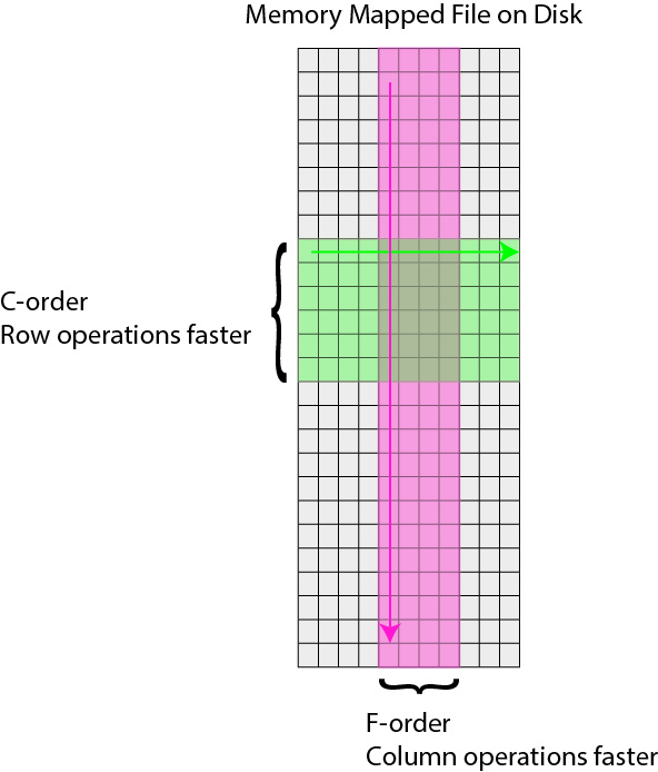
When saving memory mapped files, you can save them in F (Fortran) or C order. This determines whether the bytes will be read/written by column or by row, respectively. This is important because certain operations are much faster on C-order arrays vs F-order arrays. For motion correction, which needs to access contiguous sequences of frames (often in the middle of the movie), it is much more efficient to read and write in F order. On the other hand, when it comes to CNMF, you need to access individual pixels across the entire movie, so Caiman saves the motion-corrected movie in C-order before running CNMF.